This example graphically shows how you obtain the sin(θ) and cos(θ) plots and their ratio tan(θ) using a series of right angle triangles of Hypotenuse 1 and a Circle of Radius 1. It also gives the user some practice with their plotting with MATLAB.

Pythagorean Triple (3,4,5)

We can plot a classic 3,4,5 right angle triangle in MATLAB using the code:

%% Triangle 1 x=[0,4,4,0]; y=[0,0,3,0]; plot(x,y,'r'); xlim([-1,7]); ylim([-1,7]); axis('square'); text(0.5,0.25,'\theta'); text(3.5,0.25,'90'); text(3.5,2.25,'\gamma'); text(1.5,-0.5,'Adjacent (A)'); text(4.5,1.5,'Opposite (O)'); text(0,2,'Hypotenuse (H)');

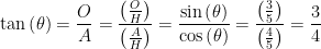
The definition of the sine from the perspective of the angle θ is the ratio of the Opposite (O) to the Hypotenuse (H) for the cosine it is the ratio of the Adjacent (A) to the Hypotenuse (H) and for the tangent it is the ratio of the Opposite (O) to the Hypotenuse (H).

$\displaystyle \sin \left( \theta \right)=\frac{O}{H}$

$\displaystyle \cos \left( \theta \right)=\frac{A}{H}$

$\displaystyle \tan \left( \theta \right)=\frac{O}{A}$

Let's have a look at these:

$\displaystyle \sin \left( \theta \right)=\frac{3}{5}$

$\displaystyle \cos \left( \theta \right)=\frac{4}{5}$

$\displaystyle \tan \left( \theta \right)=\frac{3}{4}$

Simply by definition:

$\displaystyle \tan \left( \theta \right)=\frac{O}{A}=\frac{{\left( {\frac{O}{H}} \right)}}{{\left( {\frac{A}{H}} \right)}}=\frac{{\sin \left( \theta \right)}}{{\cos \left( \theta \right)}}=\frac{{\left( {\frac{3}{5}} \right)}}{{\left( {\frac{4}{5}} \right)}}=\frac{3}{4}$

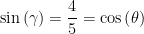
Now if look from the perspective of the angle γ then:

$\displaystyle \sin \left( \gamma \right)=\frac{4}{5}$

$\displaystyle \cos \left( \gamma \right)=\frac{3}{5}$

$\displaystyle \tan \left( \gamma \right)=\frac{4}{3}$

This means:

$\displaystyle \sin \left( \gamma \right)=\frac{4}{5}=\cos \left( \theta \right)$

$\displaystyle \cos \left( \gamma \right)=\frac{3}{5}=\sin \left( \theta \right)$

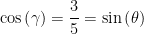
However the three sides of a triangle add up to 180 degrees. Since we are using a right angle triangle the two other angles must add up to 90 thus:

$\displaystyle \gamma =90-\theta$

It then follows:

$\displaystyle \cos \left( \theta \right)=\sin \left( {90-\theta } \right)$

$\displaystyle \sin \left( \theta \right)=\cos \left( {90-\theta } \right)$

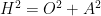
Now returning to the angle θ we have picked a right angle triangle with the sides O=3, A=4 and H=5. This triangle and all right angle triangles obey Pythagoras theorem:

$\displaystyle {{H}^{2}}={{O}^{2}}+{{A}^{2}}$

$\displaystyle {{5}^{2}}={{4}^{2}}+{{3}^{2}}$

$\displaystyle 25=25$

We can divide through by $\displaystyle {{H}^{2}}$

$\displaystyle \frac{{{{H}^{2}}}}{{{{H}^{2}}}}=\frac{{{{O}^{2}}}}{{{{H}^{2}}}}+\frac{{{{A}^{2}}}}{{{{H}^{2}}}}$

$\displaystyle 1={{\sin }^{2}}\left( \theta \right)+{{\cos }^{2}}\left( \theta \right)$

If we plug in our values we can see:

$\displaystyle 1={{\left( {\frac{4}{5}} \right)}^{2}}+{{\left( {\frac{3}{5}} \right)}^{2}}$

$\displaystyle 1=\frac{16}{{25}}+\frac{{9}}{{25}}$

$\displaystyle 1=1$

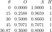
We can measure these angles using a protractor and find that θ=36.87.

If we normalise $\displaystyle H$ meaning we divide through by 5, we instead get the side lengths O=4/5, A=3/5 and H=1.

30, 60, 90 Degrees Triangle

%% Triangle 2 x=[0,3^(1/2),3^(1/2),0]; y=[0,0,1,0]; plot(x,y,'r'); xlim([-0.5,2]); ylim([-0.5,2]); axis('square'); text(0.3,0.13,'\theta'); text(1.6,0.13,'90'); text(1,0.77,'\gamma'); text(1,-0.1,'A'); text(1.8,0.5,'O'); text(0.5,0.5,'H');

Here:

$\displaystyle \theta =30$

$\displaystyle 90-\theta =60$

$\displaystyle O=1$

$\displaystyle A=\sqrt{3}$

$\displaystyle H=2$

If we normalise $\displaystyle H$ meaning we divide through by 2, we instead get the triple O=0.5, A=√3/4, and H=1.

Plotting Both Triangles Normalised with H = 1

%% Both Triangles % 3,4,5 triangle normalised so H=1 x1=[0,(4/5),(4/5),0]; y1=[0,0,(3/5),0]; % 30, 60, 90 triangle normalised so H=1 x2=[0,(3^0.5)/2,(3^0.5)/2,0]; y2=[0,0,0.5,0]; scatter(x1,y1,50,'r'); hold('on'); plot(x1,y1,'r:'); scatter(x2,y2,50,'g'); plot(x2,y2,'g:'); hold('off'); % Square Grid centred at 0,0 xlim([-1.2,1.2]); ylim([-1.2,1.2]); ax=gca; ax.XAxisLocation='origin'; ax.YAxisLocation='origin'; grid('minor'); axis('square'); xlabel('x'); ylabel('y');

We have plotted this on a grid centred at an origin. H for both triangles is 1. The end point of each triangle has an x value corresponding to the triangles Adjacent and a y value corresponding to the triangles Opposite sides. Since H=1 these are the values of sin(θ) and cos(θ) respectively.

0 Degrees – A Straight Line

Continuing with $\displaystyle H=1$ first let's see when the angle θ=0, this means that $\displaystyle A=H=1$ and $\displaystyle O=0$

%% Theta=0 O=H x=[0,1]; y=[0,0]; scatter(x,y,50,'c'); hold('on'); plot(x,y,'c'); hold('off'); % Square Grid centred at 0,0 xlim([-1.2,1.2]); ylim([-1.2,1.2]); ax=gca; ax.XAxisLocation='origin'; ax.YAxisLocation='origin'; grid('minor'); axis('square'); xlabel('x'); xlabel('y');

We can update the plots to include this additional line (θ=0).

%% Both Triangles and Line % 3,4,5 triangle normalised so H=1 x1=[0,(4/5),(4/5),0]; y1=[0,0,(3/5),0]; % 30, 60, 90 triangle normalised so H=1 x2=[0,(3^0.5)/2,(3^0.5)/2,0]; y2=[0,0,0.5,0]; % Line O=H=1 x3=[0,1]; y3=[0,0]; scatter(x1,y1,50,'r'); hold('on'); plot(x1,y1,'r:'); scatter(x2,y2,50,'g'); plot(x2,y2,'g:'); scatter(x3,y3,50,'c'); plot(x3,y3,'c:'); hold('off'); % Square Grid centred at 0,0 xlim([-1.2,1.2]); ylim([-1.2,1.2]); ax=gca; ax.XAxisLocation='origin'; ax.YAxisLocation='origin'; grid('minor'); axis('square'); xlabel('x'); ylabel('y');

45 Degree Triangle

Now let us look at what happens at a 45 degree angle:

$\displaystyle {{H}^{2}}={{O}^{2}}+{{A}^{2}}$

At 45 degrees:

$\displaystyle \cos \left( {45} \right)=\sin \left( {90-45} \right)$

$\displaystyle \sin \left( {45} \right)=\cos \left( {90-45} \right)$

And:

$\displaystyle \sin \left( {45} \right)=\cos \left( {45} \right)$

$\displaystyle \frac{O}{H}=\frac{A}{H}$

$\displaystyle H=1$

$\displaystyle O=A$

We can rewrite Pythagoras theorem:

$\displaystyle {{1}^{2}}={{O}^{2}}+{{A}^{2}}$

But:

$\displaystyle O=A$

So:

$\displaystyle {{1}^{2}}=2{{O}^{2}}$

$\displaystyle 1=2{{O}^{2}}$

$\displaystyle {{O}^{2}}=\frac{1}{2}$

$\displaystyle O=\frac{1}{{\sqrt{2}}}$

Let us plot these points:

%% Theta = 45 x=[0,(1/2^0.5),(1/2^0.5),0]; y=[0,0,(1/2^0.5),0];scatter(x,y,50,'m'); hold('on'); plot(x,y,'m:'); hold('off'); % Square Grid centred at 0,0 xlim([-1.2,1.2]); ylim([-1.2,1.2]); ax=gca; ax.XAxisLocation='origin'; ax.YAxisLocation='origin'; grid('minor'); axis('square'); xlabel('x'); ylabel('y');

We can update the plot to include this additional triangle. Try this yourself:

%% Three Triangles and Line % 3,4,5 triangle normalised so H=1 x1=[0,(4/5),(4/5),0]; y1=[0,0,(3/5),0]; % 30, 60, 90 triangle normalised so H=1 x2=[0,(3^0.5)/2,(3^0.5)/2,0]; y2=[0,0,0.5,0]; % Line O=H=1 x3=[0,1]; y3=[0,0]; x4=[0,(1/2^0.5),(1/2^0.5),0]; y4=[0,0,(1/2^0.5),0]; scatter(x1,y1,50,'r'); hold('on'); plot(x1,y1,'r:'); scatter(x2,y2,50,'g'); plot(x2,y2,'g:'); scatter(x3,y3,50,'c'); plot(x3,y3,'c:'); scatter(x4,y4,50,'m'); plot(x4,y4,'m:'); hold('off'); % Square Grid centred at 0,0 xlim([-1.2,1.2]); ylim([-1.2,1.2]); ax=gca; ax.XAxisLocation='origin'; ax.YAxisLocation='origin'; grid('minor'); axis('square'); xlabel('x'); ylabel('y');

If we update the plots to include an Arc of constant radius (Hypotenuse) of 1 we can see that the end point of each triangle lies on this Arc.

So far we have triangles for: θ=0, 30, 36.87 and 45. Let's draw the point for θ=15 and remove θ=36.87 so we are evenly spaced. For this triangle O=0.2588 and A=0.9659.

This gives us:

$\displaystyle \begin{array}{*{20}{r}} \theta & O & A & H \\ 0 & {0.0000} & {1.0000} & 1 \\ {15} & {0.2588} & {\text{0}\text{.9659}} & 1 \\ {30} & {0.5000} & {\text{0}\text{.8660}} & 1 \\ {45} & {\text{0}\text{.7071}} & {\text{0}\text{.7071}} & 1 \\ {36.87} & {0.3600} & {0.8000} & 1 \end{array}$

Angles from 45-90

From earlier we deduced:

$\displaystyle \cos \left( \theta \right)=\sin \left( {90-\theta } \right)$

We have drawn the triangle at θ=36.87, we can also redraw this triangle starting on the y axis (90) and working back from 90 to subtract θ. This gives 90-θ=90-36.87=53.13 (the angle from the x-axis that we are interested in). In other words this is the transpose of the first triangle. Draw the normalised 3,4,5 sided triangle and it's transpose.

%% Triangle and Triangle Transpose % 3,4,5 triangle normalised so H=1 x=[0,(4/5),(4/5),0]; y=[0,0,(3/5),0]; scatter(x,y,50,'r'); hold('on'); plot(x,y,'r:'); scatter(y,x,50,'r'); plot(y,x,'r:'); hold('off'); % Square Grid centred at 0,0 xlim([-1.2,1.2]); ylim([-1.2,1.2]); ax=gca; ax.XAxisLocation='origin'; ax.YAxisLocation='origin'; grid('minor'); axis('square'); xlabel('x'); ylabel('y');

We can see that the dimensions of these two triangles are identical however $\displaystyle O$ and $\displaystyle A$ are flipped from the original to second triangle:

Oθ1=Aθ2

Aθ1=Oθ2

Apply this knowledge to θ=0, 15, 30 and 45 and plot the results.

Or:

$\displaystyle \begin{array}{*{20}{r}} \theta & O & A & H \\ 0 & {0.0000} & {1.0000} & 1 \\ {15} & {0.2588} & {0.9659} & 1 \\ {30} & {0.5000} & {0.8660} & 1 \\ {45} & {0.7071} & {0.7071} & 1 \\ {60} & {0.8660} & {0.5000} & 1 \\ {75} & {0.9659} & {0.2588} & 1 \\ {90} & {1.0000} & {0.0000} & 1 \\ {36.87} & {0.3600} & {0.8000} & 1 \\ {53.13} & {0.8000} & {0.3600} & 1 \end{array}$

Looking at the Rest of the Circle

We have drawn the triangle at θ=36.87. What happens when you change the sign of the x-value?

Try this yourself:

%% Triangle (-x) % 3,4,5 triangle normalised so H=1 x=[0,(4/5),(4/5),0]; y=[0,0,(3/5),0]; scatter(-x,y,50,'r'); hold('on'); plot(-x,y,'r:'); hold('off'); % Square Grid centred at 0,0 xlim([-1.2,1.2]); ylim([-1.2,1.2]); ax=gca; ax.XAxisLocation='origin'; ax.YAxisLocation='origin'; grid('minor'); axis('square'); xlabel('x'); ylabel('y');

We are taken to the second quadrant, note as we are drawing a point on a circle with radius 1, this mirror image in x is still on the circle.

What happens if this time we change the sign of the x and y value. Try this yourself:

%% Triangle (-x and -y) % 3,4,5 triangle normalised so H=1 x=[0,(4/5),(4/5),0]; y=[0,0,(3/5),0]; scatter(-x,-y,50,'r'); hold('on'); plot(-x,-y,'r:'); hold('off'); % Square Grid centred at 0,0 xlim([-1.2,1.2]); ylim([-1.2,1.2]); ax=gca; ax.XAxisLocation='origin'; ax.YAxisLocation='origin'; grid('minor'); axis('square'); xlabel('x'); ylabel('y');

We are taken to the third quadrant, note as we are drawing a point on a circle with radius 1, this mirror image in x and y is still on the circle.

What happens if this time we change the sign of only the y value. Try this yourself:

%% Triangle (x and -y) % 3,4,5 triangle normalised so H=1 x=[0,(4/5),(4/5),0]; y=[0,0,(3/5),0]; scatter(x,-y,50,'r'); hold('on'); plot(x,-y,'r:'); hold('off'); % Square Grid centred at 0,0 xlim([-1.2,1.2]); ylim([-1.2,1.2]); ax=gca; ax.XAxisLocation='origin'; ax.YAxisLocation='origin'; grid('minor'); axis('square'); xlabel('x'); ylabel('y');

We are taken to the fourth quadrant, note as we are drawing a point on a circle with radius 1, this mirror image in y is still on the circle.

Therefore:

Quarter 1:

Quarter 2:

$\displaystyle \begin{array}{*{20}{r}} \theta & O & A & H \\ {180} & {0.0000} & {-1.0000} & 1 \\ {165} & {0.2588} & {-0.9659} & 1 \\ {150} & {0.5000} & {-0.8660} & 1 \\ {135} & {0.7071} & {-0.7071} & 1 \\ {120} & {0.8660} & {-0.5000} & 1 \\ {105} & {0.9659} & {-0.2588} & 1 \\ {90} & {1.0000} & {-0.0000} & 1 \\ {143.13} & {0.3600} & {-0.8000} & 1 \\ {126.7} & {0.8000} & {-0.3600} & 1 \end{array}$

Quarter 3:

$\displaystyle \begin{array}{*{20}{r}} \theta & O & A & H \\ {180} & {-0.0000} & {-1.0000} & 1 \\ {195} & {-0.2588} & {-0.9659} & 1 \\ {210} & {-0.5000} & {-0.8660} & 1 \\ {225} & {-0.7071} & {-0.7071} & 1 \\ {240} & {-0.8660} & {-0.5000} & 1 \\ {255} & {-0.9659} & {-0.2588} & 1 \\ {270} & {-1.0000} & {-0.0000} & 1 \\ {143.13} & {-0.3600} & {-0.8000} & 1 \\ {233.13} & {-0.8000} & {-0.3600} & 1 \end{array}$

Quarter 4:

$\displaystyle \begin{array}{*{20}{r}} \theta & O & A & H \\ {360} & {-0.0000} & {1.0000} & 1 \\ {345} & {-0.2588} & {0.9659} & 1 \\ {330} & {-0.5000} & {0.8660} & 1 \\ {315} & {-0.7071} & {0.7071} & 1 \\ {300} & {-0.8660} & {0.5000} & 1 \\ {285} & {-0.9659} & {0.2588} & 1 \\ {270} & {-1.0000} & {0.0000} & 1 \\ {323.13} & {-0.3600} & {0.8000} & 1 \\ {306.87} & {-0.8000} & {0.3600} & 1 \end{array}$

This means from the 4 points we calculated from the line (θ=0) and 3 triangles with θ=15, 30 and 45 respectively using symmetry we have obtained 24 points which covers the full circle and is crude enough to get a first hand approximation of the sine, cosine and tangent. Try to plot this:

%% First Quarter: 0:15:45 Degrees % Line \theta=15 x0=[0,1]; y0=[0,0]; % Line \theta=15 x15=[0,0.9659,0.9659,0]; y15=[0,0,0.2588,0];
% Line \theta=30 x30=[0,(3^0.5)/2,(3^0.5)/2,0]; y30=[0,0,0.5,0];% Line \theta=45 x45=[0,(1/2^0.5),(1/2^0.5),0]; y45=[0,0,(1/2^0.5),0]; scatter(x0,y0,50,'c'); hold('on'); plot(x0,y0,'c:');scatter(-x0,y0,50,'c');
plot(-x0,y0,'c:');scatter(-x0,-y0,50,'c'); plot(-x0,-y0,'c:'); scatter(x0,-y0,50,'c'); plot(x0,-y0,'c:'); scatter(y0,x0,50,'c'); plot(y0,x0,'c:');scatter(y0,-x0,50,'c'); plot(y0,-x0,'c:'); scatter(-y0,-x0,50,'c'); plot(-y0,-x0,'c:'); scatter(-y0,x0,50,'c'); plot(-y0,x0,'c:'); scatter(x15,y15,50,'b'); plot(x15,y15,'b:'); scatter(-x15,y15,50,'b'); plot(-x15,y15,'b:'); scatter(-x15,-y15,50,'b'); plot(-x15,-y15,'b:'); scatter(x15,-y15,50,'b'); plot(x15,-y15,'b:'); scatter(y15,x15,50,'b'); plot(y15,x15,'b:'); scatter(y15,-x15,50,'b'); plot(y15,-x15,'b:'); scatter(-y15,-x15,50,'b'); plot(-y15,-x15,'b:'); scatter(-y15,x15,50,'b'); plot(-y15,x15,'b:'); scatter(x30,y30,50,'g'); plot(x30,y30,'g:'); scatter(-x30,y30,50,'g'); plot(-x30,y30,'g:'); scatter(-x30,-y30,50,'g'); plot(-x30,-y30,'g:'); scatter(x30,-y30,50,'g'); plot(x30,-y30,'g:'); scatter(y30,x30,50,'g'); plot(y30,x30,'g:'); scatter(y30,-x30,50,'g'); plot(y30,-x30,'g:'); scatter(-y30,-x30,50,'g'); plot(-y30,-x30,'g:'); scatter(-y30,x30,50,'g'); plot(-y30,x30,'g:');scatter(x45,y45,50,'m'); plot(x45,y45,'m:'); scatter(-x45,y45,50,'m'); plot(-x45,y45,'m:'); scatter(-x45,-y45,50,'m'); plot(-x45,-y45,'m:'); scatter(x45,-y45,50,'m'); plot(x45,-y45,'m:'); scatter(y45,x45,50,'m'); plot(y45,x45,'m:'); scatter(y45,-x45,50,'m'); plot(y45,-x45,'m:'); scatter(-y45,-x45,50,'m'); plot(-y45,-x45,'m:'); scatter(-y45,x45,50,'m'); plot(-y45,x45,'m:'); hold('off'); % Square Grid centred at 0,0 xlim([-1.2,1.2]); ylim([-1.2,1.2]); ax=gca; ax.XAxisLocation='origin'; ax.YAxisLocation='origin'; grid('minor'); axis('square'); xlabel('x'); ylabel('y');

Plotting the sin, cos and tan functions

We can plot $\displaystyle O$ with respect to $\displaystyle \theta$ and because $\displaystyle H=1$ this is the sin( $\displaystyle \theta$ ) likewise we can plot $\displaystyle A$ with respect to $\displaystyle \theta$ and because $\displaystyle H=1$ this is the cos( $\displaystyle \theta$ ). Moreover $\displaystyle \tan \left( \theta \right)$ is the ratio of these two values. Try this yourself.

%% Data % Angle, sin(\theta), cos(\theta), tan(\theta) angle2=[0:15:360]'; sin2=[0;0.2588;0.5;0.7071;0.866;0.9659;1;0.9659;0.8660;0.7071;0.5;0.2588;0;-0.2588;-0.5;-0.707;-0.866;-0.9659;-1;-0.9659;-0.866;-0.707;-0.5;-0.2588;0]; cos2=[1;0.9659;0.8660;0.7071;0.5;0.2588;0;-0.2588;-0.5;-0.707;-0.866;-0.9659;-1;-0.9659;-0.866;-0.707;-0.5;-0.2588;0;0.2588;0.5;0.7071;0.866;0.9659;1]; tan2=sin2./cos2; data=table(angle2,sin2,cos2,tan2); clear angle2; clear sin2; clear cos2; clear tan2; % Data for Lines x=[0,360]; y=[0,0]; x2a=[90,90]; x2b=[180,180]; x2c=[270,270]; y2=[-1,1]; y2a=[-4,4]; %% figure(1) sin(\theta) figure(1); scatter(data.angle2,data.sin2,50,'r','fill'); hold('on'); plot(x,y,'k'); plot(x2a,y2,'k'); plot(x2b,y2,'k'); plot(x2c,y2,'k'); hold('off'); grid('minor'); xlabel('\theta'); ylabel('O=O/H=sin(\theta)'); xlim([0,360]); set(gca,'Box',1); %% figure(2) cos(\theta) figure(2); scatter(data.angle2,data.cos2,50,'r','fill'); hold('on'); plot(x,y,'k'); plot(x2a,y2,'k'); plot(x2b,y2,'k'); plot(x2c,y2,'k'); hold('off'); grid('minor'); xlabel('\theta'); ylabel('A=A/H=cos(\theta)'); xlim([0,360]); set(gca,'Box',1); %% figure(3) tan(\theta) figure(3); scatter(data.angle2,data.tan2,50,'r','fill'); hold('on'); plot(x,y,'k'); plot(x2a,y2a,'k'); plot(x2b,y2a,'k'); plot(x2c,y2a,'k'); hold('off'); grid('minor'); xlabel('\theta'); ylabel('O/A=sin(\theta)/cos(\theta)=tan(\theta)'); xlim([0,360]); ylim([-4,4]); set(gca,'Box',1);

Plot of O=O/H=sin(θ) as H=1 versus θ.

Plot of A=A/H=cos(θ) as H=1 versus θ. Note that the sin(θ-90)=cos(θ) as expected: the cos(θ) plot is identical in form to the sin(θ) plot but out of phase by 90.

Plot of A=O/A=sin(θ)/cos(θ)=tan(θ), the ratio of the two plots above.

A Schematic of the Steps we Just Carried Out

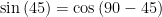
Plot a circle of radius one. Draw lines until you reach the circle (radius 1) at angles 0,15,30 and 45:

From these angles exploit the fact that sin(θ)=cos(90-θ) and meaning you can transpose the O (y) and A (x) values to complete the arc up until 90.

Next exploit the fact that you are plotting on a circle and the second quadrant is mirrored in x (-x and +y).

Next exploit the fact that you are plotting on a circle and the third quadrant is mirrored in x and y (-x and -y).

Finally exploit the fact that you are plotting on a circle and the third quadrant is mirrored in y only (x and -y).

These functions are cyclic, meaning if you go around the circle again you will get the same graph again. MATLAB has the following inbuilt functions that work with angles in Degrees:

sind(deg)
cosd(deg)
tand(deg)

Use them to make a plot of sind and cosd for angles from 0 to 1080 degrees. You should have both of these on the same plot with a legend, sind should have a blue line and cosd should have a red line.

%% plot using sind and cosd % Data t1=[0:1080]'; y1=sind(t1); y2=cosd(t1); % Plots plot(t1,y1,'color','r','LineWidth',2); hold('on'); plot(t1,y2,'color','b','LineWidth',2); hold('off'); xlabel('\theta in Degrees'); grid('minor'); xlim([0,1080]); legend('sind(\theta)','cosd(\theta)','Location','NorthEast');

And the following return an angle in Degrees:

asind(ratio)
acosd(ratio)
asind(ratio)

Use these to verify the angle of the 3 by 4 by 5 triangle:

asind(3/5)=36.8699
acosd(4/5)=36.8699
asind(3/4)=36.8699

Trigonometry – sin and cos

Pythagorean Triple (3,4,5)

30, 60, 90 Degrees Triangle

Plotting Both Triangles Normalised with H = 1

0 Degrees – A Straight Line

45 Degree Triangle

Angles from 45-90

Looking at the Rest of the Circle

Plotting the sin, cos and tan functions

A Schematic of the Steps we Just Carried Out

Like this:

Leave a ReplyCancel reply

Pythagorean Triple (3,4,5)

30, 60, 90 Degrees Triangle

Plotting Both Triangles Normalised with H = 1

0 Degrees – A Straight Line

45 Degree Triangle

Angles from 45-90

Looking at the Rest of the Circle

Plotting the sin, cos and tan functions

A Schematic of the Steps we Just Carried Out

Share this:

Like this:

Leave a ReplyCancel reply