Plotting

 

figure(1);
scatter(rocket.t,rocket.v,100,'fill');
grid('minor'):
xlabel('t');
ylabel('v');

Contents

Detailed Interpolation of a Single Point

The Interpolation Functions interp1

Detailed Interpolation of a Single Point

Suppose we have a rocket and have recorded it's speed during the list of times.

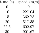
And we want to know it's speed at time t=16 s. There are a number of ways we can estimate this value or interpolate this value from the given data.

Nearest Point Interpolation (1 data point)

Simply by looking at the data we can see that the nearest time point to t=16 s is t=15 s.

We can take the speed at t=15 s and use it as a first hand estimate for the speed at t=16 s and this is known as single point interpolation.

St16=St15
St16=362.78

Linear Interpolation (2 data points)

Suppose we want to be a bit more accurate we can instead take two points and calculate the equation for a line. We can then plug in our x data point and use the equation of the straight line to estimate our unknown y data point. Looking at the data for t=16 s the nearest two time points are t=15 s and t=20 s.

The equation for a straight line is:

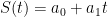
For two times we can write this out in matrix form:

Now we can substitute in the known values:

We can save the known data as variables S and T:

S=[362.78;517.35]

T=[1,15;1,20]

And call the unknown variable U:

We know that:

However we want to solve for U. We can get U on it's own by multiplying throughout by the inverse matrix of T:

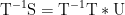
Since a matrix multiplied by it's inverse gives the identity matrix and a matrix multipied by the identity matrix gets unchanged:

Which can be reordered:

Thus to solve for U we need the inverse matrix of T:

This can be calculated using the function Minv=inv(M)

Tinv=inv(T)

Thus we can get the unknown coefficients of U using:

U=Tinv*S

i.e. in the limits of 15<t<20 a0=-100.93 and a1=30.914

Instead of using the inverse matrix we could also use left division

U=T\S

Now that we have the coefficients we can calculate the S(16)

St16=[1,16]*U

We can check the equation using the known data:

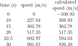
Unsurprisingly the values at the limits t=15 and t=20 give exact matches. There is a slight deviation just outside this interval and a massive deviation substantially away from this interval.

Quadratic Interpolation (3 data points)

Suppose we want to be a bit more accurate we can instead take three points and calculate a quadratic equation. We can then plug in our x data point and use the quadratic equation to estimate our unknown y data point. Looking at the data for t=16 s the nearest three time points are t= 10 s, t=15 s and t=20 s.

The equation for a quadratic function is:

For three times we can write this out in matrix form:

Now we can substitute in the known values:

We can save the known data as variables S and T:

S=[227.04;362.78;517.35]

T=[1,10,10^2;1,15,15^2;1,20,20^2]

And call the unknown variable U:

To solve for U we use:

U=T\S

i.e. in the limits of 10<t<20 a0=12.05, a1=17.733 and a2=0.3766

Now that we have the coefficients we can calculate the S(16)

St16=[1,16,16^2]*U

Cubic Interpolation (4 data points)

Suppose we want to be a bit more accurate we can instead take four points and calculate a cubic equation. We can then plug in our x data point and use the cubic equation to estimate our unknown y data point. Looking at the data for t=16 s the nearest three time points are t= 10 s, t=15 s, t=20 s and t=22.5 s.

The equation for a cubic function is:

For four times we can write this out in matrix form:

Now we can substitute in the known values:

We can save the known data as variables S and T:

S=[227.04;362.78;517.35;602.97]

T=[1,10,10^2,10^3;1,15,15^2,15^3;1,20,20^2,20^3;1,22.5,22.5^2,22.5^3]

And call the unknown variable U:

To solve for U we use:

U=T\S

i.e. in the limits of 10<t<22.5 a0=4.254, a1=21.2655333, a2=0.13204 and a3=0.0054347

Now that we have the coefficients we can calculate the S(16)

St16=[1,16,16^2,16^3]*U

Comparison

We can compare our interpolation for t=16 using the four different methods. As we can see when we are interpolating with higher order polynomials the result begins to converge as expected:

Interpolation of a Data Set

As we seen it is quite involved interpolating the data for a single data point. If we want to interpolate 100's or even 1000's of data points manually going through them all like above it would take all day. Luckily Octave/MATLAB have inbuilt interpolation functions.

intery=interp1(originalx,originaly,xdatapoints,'Method')

We can type in the data using Octave/MATLAB.

[code language="matlab"]

data=[0,0;
10,227.04;
15,362.78;
20,517.35;
22.5,602.97;
30,901.67]

[/code]

We could also use Excel to copy and paste in the data. In MATLAB which is more polished, we can directly go to the variable editor, right click it and create a new variable and then name accordingly. This option isn't available in Octave however we can quickly create a variable, assign in to a scalar and then copy and paste in a matrix in the variable editor.

For instance typing in:

data=1;

Then clicking the new variable data in the workspace to open it up in the variable editor:

We can right click the top cell of data in the variable editor and we can right click Paste Table to copy the Excel Data through to Octave:

Now we have our data variable:

Next we need to make the new x data. For this I am going to make a new variable called dataint and I want the first column to go from 1 to 30. Here logical indexing is used when creating the variable dataint. The (:,1) means we are creating data in all rows but using the first column. The [1:30]' is a column vector ranging from 1 to 30 in steps of 1. If you are unsure about logical indexing see my earlier guide Introduction to Arrays.

dataint(:,1)=[1:30]'

Now we are looking to interpolate the data:

intery=interp1(originalx,originaly,xdatapoints,'Method')

Our original x data originalx is the first column of data our original y data originaly is the second column of data

originalx=data(:,1)

originaly=data(:,2)

Our x datapoints xdatapoints are the first column in dataint

xdatapoints=dataint(:,1)

We will start with Nearest Interpolation meaning instead of typing in 'Method' we type in 'Nearest'. We can now get intery:

intery=interp1(originalx,originaly,xdatapoints,'Nearest')

We can clear up our code here:

intery=interp1(originalx,originaly,xdatapoints,'Nearest')

By substituting these in directly:

originalx=data(:,2)

originaly=data(:,2)

xdatapoints=dataint(:,1)

This becomes

intery=interp1(data(:,1),data(:,2),dataint(:,1),'Nearest')

Now it is more likely we want the y data to be alongside the xdatapoints so instead of having the separate output variable intery we can add it as a second column to dataint by using:

dataint(:,2)=interp1(data(:,1),data(:,2),dataint(:,1),'Nearest')

We can press the [↑] key to get our last line of code and easily modify the line of code to print linear interpolated data to column 3. For linear interpolation the method is 'Linear':

dataint(:,3)=interp1(data(:,1),data(:,2),dataint(:,1),'Linear')

MATLAB/Octave's interp1 function doesn't have an inbuilt quadratic interpolation so I will go directly to cubic interpolation and here the method is 'Pchip' , this time I want the data in the 4th column.

dataint(:,4)=interp1(data(:,1),data(:,2),dataint(:,1),'Pchip')

Since we were interested at the value at t=16 which is the 16th row we can output the 16th row into the command window:

t16row=dataint(16,:)

These are very similar to the values manually calculated, the differences are likely due to rounding.

The code above can be cleared up and put in a script file.

[code language="matlab"]
% Data
data=[0,0;
10,227.04;
15,362.78;
20,517.35;
22.5,602.97;
30,901.67];

% Lower and Upper Limits for interpolation
m=1;
n=30;

% Interpolation Spreadsheet
dataint(:,1)=[m:n]';
dataint(:,2)=interp1(data(:,1),data(:,2),dataint(:,1),'Nearest');
dataint(:,3)=interp1(data(:,1),data(:,2),dataint(:,1),'Linear');
dataint(:,4)=interp1(data(:,1),data(:,2),dataint(:,1),'Pchip');

[/code]