Introduction

This example will look at a simple 4 by 4 magic square, shown below. Logical indexing and the sum function (with a single input argument) will be used to look at the sum of each row, each column, the diagonal and antidiagonal in the magic square. For this you need to be comfortable with running Octave/MATLAB and need to understand how to measure the size of an array and use logical indexing. See my guide Introduction to Arrays in Octave and MATLAB if you need a refresher.

As computing the sum of rows for example is an operation being carried out for a sequence of events, it can be automated by using a for loop.

Note much of the steps below can be simplified by inputting multiple input arguments into the sum function and using the diag, flip, flipud and fliplr functions however the main point of this written guide is to introduce the powerful tool of for loops using a simple example.

---

Create a Magic Square

Working with a Magic Square is a good way to practice working with logical indexing of arrays and hence explore the concept behind creating a for loop. A Magic Square can be created using the magic function, the input argument will be the size of the square, in this case I will use 4:

% The magic square
M=magic(4)

---

Look at a Matrix Dimensions

Although we know the size of the square is 4 by 4, let's use the size function to prescribe the magic squares dimensions to the variables m (number of rows) and n (number of columns).

[m,n]=size(M)

---

Initialisation of Output Array – sumrow

To begin we should initialise our column vector which contains a column of sums for each row. This can be done using the zeros function, the inputs for the zero function are m and 1 as we are looking for a column vector that has m rows (and 1 column)

sumrow=zeros(m,1)

Initialisation in essence, creates an array with the desired variable name and desired final dimensions. In this case the column of sums which is going to be m rows by 1 column. At initialisation we don't know the values of each element in the array so we prescribe each value to 0. We can sub-sequentially use logical indexing to replace each of the values in this column vector.

---

Look at the Sum of the First Row

Let's look at the first row:

sumrow(1)=sum(M(1,[1:n]))

This can also be abbreviated as:

sumrow(1)=sum(M(1,:))

What we are essentially doing on the left hand side is using logical indexing to prescribe the value to the 1st index of the column vector sumrow. To the right hand side we are using logical indexing to create a row vector and inputting this row vector into the sum function. The scalar calculated from the sum function is prescribed to the 1st index of the column vector sumrow.

---

Look at the Sum of Each Row

We can now manually go through the same process by looking at each row in turn.

sumrow(1)=sum(M(1,:))

sumrow(2)=sum(M(2,:))

sumrow(3)=sum(M(3,:))

sumrow(4)=sum(M(4,:))

---

Look at the Sum of Each Row in a For Loop

Note how we used the following lines of code, these all look identical with exception to the part highlighted in red

sumrow(1)=sum(M(1,:))

sumrow(2)=sum(M(2,:))

sumrow(3)=sum(M(3,:))

sumrow(4)=sum(M(4,:))

These can be combined together using a for loop. The for loop has to start with for followed by some condition which increments from a starting point in steps until an ending point. We use end to end the for loop.

for condition

end

We need to create a condition that increments during each iteration of the for loop, let's call it A. From the above, the only change in the line of code is the value in red, we need to set this to A and have A to equal the value shown above for each iteration of a for loop. Thus we know that A starts at 1, then steps up by increments of 1 to 2, 3 and ends at m which in this case is 4. This condition is met when A=[1:m]', the transpose is used because we are looking for a column vector, containing the sum value of each row.

for A=[1:m]'

end

Now we can rewrite:

sumrow(1)=sum(M(1,:))

sumrow(2)=sum(M(2,:))

sumrow(3)=sum(M(3,:))

sumrow(4)=sum(M(4,:))

As a single line in terms of A:

sumrow(A)=sum(M(A,:))

To the left hand side we are embedding into the Ath index of the column vector sumrow. To the right hand side we are calculating the sum of each row of M.

This line of code should be embedded within the for loop. The convention is to indent any code embedded in a loop therefore it will have the form:

for  A=[1:m]'

    sumrow(A)=sum(M(A,:))

end

When running this code, we will therefore start with the following

sumrow=zeros(m,1)

The code

for A=[1:m]'

    sumrow(A)=sum(M(A,:))

end

In the first step will become

for A=1

    sumrow(1)=sum(M(1,:))

end

In the second step will become

for A=2

    sumrow(2)=sum(M(2,:))

end

In the third step it will become

for A=3

    sumrow(3)=sum(M(3,:))

end

In the mth step, it will become

for A=m

    sumrow(m)=sum(M(m,:))

end

This gives us the m by 1 column vector of the sums of the rows of the magic square respectively.

---

Initialisation of Output Array – sumcol

Now we can follow a similar procedure. This time looking at the sums of each column which will give us a row vector called sumcol. To begin we should initialise our row vector which contains a row of sums for each column. This can be done using the zeros function, the inputs for the zero function are 1 and n as we are looking for a row vector that has (1 row and) m columns

sumrow=zeros(1,n)

Initialisation in essence, creates an array with the desired variable name and desired final dimensions. In this case the column of sums which is going to be m rows by 1 column. At initialisation we don't know the values of each element in the array so we prescribe each value to 0. We can sub-sequentially use logical indexing to replace each of the values in this column vector.

---

Look at the Sum of the First Column

Let's look at the first column

sumcol(1)=sum(M([1:m]',1))

This can also be abbreviated as:

sumcol(1)=sum(M(:,1))

What we are essentially doing on the left hand side is using logical indexing to prescribe the value to the 1st index of the row vector sumcol. To the right hand side we are using logical indexing to create a column vector and inputting this column vector into the sum function. The scalar calculated from the sum function is prescribed to the 1st index of the row vector sumcol.

---

Look at the Sum of Each Column

sumcol(1)=sum(M(:,1))

sumcol(2)=sum(M(:,2))

sumcol(3)=sum(M(:,3))

sumcol(4)=sum(M(:,4))

---

Look at the Sum of Each Column using a For Loop

Note how we used the following lines of code, these all look identical with exception to the part highlighted in orange

sumcol(1)=sum(M(:,1))

sumcol(2)=sum(M(:,2))

sumcol(3)=sum(M(:,3))

sumcol(4)=sum(M(:,4))

These can be combined together using a for loop. Once again we need to create a condition which has some starting value and increments in steps until a final value, let’s call it B. We know that B starts at 1, then steps up by increments of 1 to 2, 3 and ends at 4. In other words the row vector B=[1:n]. We use a row vector as we are looking to create a row vector which contains the sum of each columns. Therefore the for loop becomes:

for B=[1:n]

    sumcol(B)=sum(M(:,B))

end

To the left hand side we are embedding into the Bth index of the row vector sumcol. To the right hand side we are calculating the sum of each col of M. This line of code should once again be embedded within the for loop. Once again we follow the convention is to indent any code embedded in a loop.

When running this code, we will therefore start with the following

sumcol=zeros(1,n)

The code

for B=[1:n]

    sumcol(B)=sum(M(:,B))

end

In the first step will become

for B=1

    sumcol(1)=sum(M(:,1))

end

In the second step will become

for B=2

    sumcol(2)=sum(M(:,2))

end

In the third step will become

for B=3

    sumcol(3)=sum(M(:,3))

end

In the nth step it will become

for B=n

    sumcol(n)=sum(M(:,n))

end

This gives us the 1 by n row vector of the sums of the columns of the magic square respectively.

---

Initialisation of Output Array – diag

It may not be immediately obvious but we can use the same method to look at the sum of the diagonal. To do this we need to turn the diagonal into a row (or column) vector, we will use a row vector.

Let's first initialise the row vector diag using

diag=zeros(1,n)

---

Create diag row vector using a For Loop

Manually the diagonal has the position

diag(1)=M(1,1)

diag(2)=M(2,2)

diag(3)=M(3,3)

diag(4)=M(4,4)

We can create the above by using the for loop. We need to create a condition which has some starting value and increments in steps until an end value, let’s call it C. We know that C starts at 1, then steps up by increments of 1 to 2, 3 and ends at n=4 in this case. In other words the column vector C=[1:n]. Therefore the for loop becomes:

for C=1:n
     diag(C)=M(C,C)
end

To the left hand side we are embedding into the Cth index of the row vector diag. To the right hand side we are indexing the Cth index into both the row and column. This line of code should once again be embedded within the for loop. Recalling the convention is to indent any code embedded in a loop.

When running this code, we will therefore start with the following

diag=zeros(1,n)

The code

for C=1:n
     diag(C)=M(C,C)
end

In the first step will become

for C=1
     diag(1)=M(1,1)
end

In the second step will become

for C=2
     diag(2)=M(2,2)
end

In the third step will become

for C=3
     diag(3)=M(3,3)
end

In the nth step will become

for C=n
     diag(n)=M(n,n)
end

---

Calculate the sum of the diag

Now that we have the diag as a row vector, calculating the sum of it is fairly straight forward.

sumdiag=sum(diag)

---

Initialisation of Output Array – antidiag

We can use the same method to look at the sum of the antidiagonal. To do this we need to turn the antidiagonal into a row (or column) vector, we will use a row vector.

Let's first initialise the row vector diag using

antidiag=zeros(1,n)

---

Create antidiag row vector using a For Loop

Manually the diagonal has the position

antidiag(1)=M(1,4)

antidiag(2)=M(2,3)

antidiag(3)=M(3,2)

antidiag(4)=M(4,1)

We can create the above by using the for loop. We need to create a condition which has some starting value and increments in steps to a final value, let’s call it D. We know that D starts at 1, then steps up by increments of 1 to 2, 3 and ends at n=4 in this case. In other words the column vector D=[1:n]. It is obvious how to calculate the index on the left hand side and the row index on the right hand side in terms of D but in order to make a loop we also need to define the column index in terms of D. We have the size of the matrix as m by n and we know we are lowering our index as D increases. If we use n-D, this will give us 3,2,1,0 however what we want is 4,3,2,1 therefore we must use n+1-D. The +1 is required when indexing the column as we index the matrix from 1 upwards and not from 0 upwards.

antidiag(1)=M(1,n+1-1)

antidiag(2)=M(2,n+1-2)

antidiag(3)=M(3,n+1-3)

antidiag(n)=M(n,n+1-n)

Therefore the for loop becomes

for D=1:n
     antidiag(D)=M(D,n+1-D)
end

To the left hand side we are embedding into the Dth index of the row vector diag. To the right hand side we are indexing the Dth index into the row. For the antidiag, when the row=1, the column=end and when the row=end, the column=1. Introducing a variable D=1:n we know that the antidiag lies on M(D,n-D+1). This line of code should once again be embedded within the for loop. Once again we follow the convention to indent any code embedded in a loop. When running this code, we will therefore start with the following

The code

for D=1:n
     antidiag(D)=M(D,n+1-D)
end

In the first step will become

for D=1
     antidiag(1)=M(1,n+1-1)
end

Which gives the first element of the antidiagonal (in the first row)

for D=1
     antidiag(1)=M(1,n)
end

In the second step will become

for D=2
     antidiag(2)=M(2,n+1-2)
end

Which gives the second element of the antidiagonal (in the second row)

for D=2
     antidiag(2)=M(2,n-1)
end

In the third step will become

for D=3
     antidiag(3)=M(3,n+1-3)
end

Which gives the third element of the antidiagonal (in the third row)

for D=3
     antidiag(3)=M(3,n-2)
end

In the nth step will become

for D=n
     antidiag(n)=M(n,n+1-n)
end

However n=end, Which gives the last element of the antidiagonal

for D=n
     antidiag(n)=M(n,1)
end

---

Calculate the sum of the diag

Now that we have the antidiag as a row vector, calculating the sum of it is fairly straight forward.

sumantidiag=sum(antidiag)

---

Script to Measure Sum of All Sides of a Magic Square

[code language="matlab"]
% Create a Magic Square
M=magic(4)
% Get the Size of the Magic Square
[m,n]=size(M)
%
% The sums of the rows
% Initialisation of the column vector sumrow
sumrow=zeros(m,1);
% For Loop Measuring the sums of the rows
for A=[1:m]'
sumrow(A)=sum(M(A,:));
end
sumrow
%
% The sums of the cols
% Initialisation of the row vector sumcol
sumcol=zeros(1,n);
% For Loop Measuring the sums of the columns
for B=1:n
sumcol(B)=sum(M(B,:));
end
sumcol
%
% The sum of the diagonal
% Initialisation of the diagonal as a row vector
diag=zeros(1,n);
% For Loop computing the diagonal as a row vector
for C=1:n
diag(C)=M(C,C);
end
% The sum of the diagonal
sumdiag=sum(diag)
%
% The sum of the antidiagonal
% Intialisation of the antidiagonal as a row vector
antidiag=zeros(1,n);
% For Loop computing the antidiagonal as a row vector
for D=1:n
antidiag(D)=M(D,n+1-D);
end
% The sum of the antidiagonal
sumantidiag=sum(antidiag)
[/code]

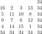
We used a relatively small Magic Square that was 4 by 4 where it is possible to visually manually calculate the sum of the rows, the sum of the columns and the sum of the diagonals i.e.

We can however change the code above to look at a far more complicated 9 by 9 magic square by changing the 4 in line 2 to a 9:

---