Python, NumPy, SciPy and MatPlotLib Interpolation

Table of contents

Tutorial Video
Perquisites

Data Points
Manual Interpolation of a Single Point
Interpolation of Multiple Data Points using an Interpolation Function

Tutorial Video

Perquisites

We will need the numpy, scipy and matplotlib.pylot libraries:

# Perquisites
import numpy as np
import scipy as sp
import matplotlib.pyplot as plt
import scipy.interpolate

Data Points

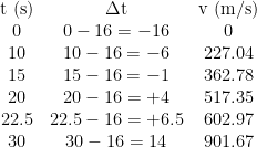
Supposing we have recorded the speed of a rocket at the following 6 time points:

$\displaystyle \begin{array}{*{20}{c}} {\text{t (s)}} & {\text{v (m/s)}} \\ 0 & 0 \\ {10} & {227.04} \\ {15} & {362.78} \\ {20} & {517.35} \\ {22.5} & {602.97} \\ {30} & {901.67} \end{array}$

We can create NumPy arrays from the data:

# Perquisites
import numpy as np
import scipy as sp
import matplotlib.pyplot as plt
import scipy.interpolate
# Create Data
t=np.array([0,10,15,20,22.5,30])
v=np.array([0,227.04,362.78,517.35,602.97,901.67])

To plot the figure we can use:

# Perquisites
import numpy as np
import scipy as sp
import matplotlib.pyplot as plt
import scipy.interpolate
# Create Data
t=np.array([0,10,15,20,22.5,30])
v=np.array([0,227.04,362.78,517.35,602.97,901.67])
# Plot Data
plt.close('all')
plt.figure(1)
plt.grid(axis='both',which='major',color=[166/255,166/255,166/255], linestyle='-', linewidth=2)
plt.minorticks_on()
plt.grid(axis='both',which='minor',color=[166/255,166/255,166/255], linestyle=':', linewidth=1)
plt.xlabel('time (s)')         
plt.ylabel('velocity (m/s)')        
plt.title('Projectile of a Rocket') 
plt.scatter(t,v,50,[255/255,0/255,0/255],label='original data')
plt.legend(loc='upper left')

Manual Interpolation of a Single Point

Supposing we want to know the velocity at t=16 s, how can we estimate it from the data provided?

# Perquisites
import numpy as np
import scipy as sp
import matplotlib.pyplot as plt
import scipy.interpolate
# Create Data
t=np.array([0,10,15,20,22.5,30])
v=np.array([0,227.04,362.78,517.35,602.97,901.67])
# Plot Data
plt.close('all')
plt.figure(1)
plt.grid(axis='both',which='major',color=[166/255,166/255,166/255], linestyle='-', linewidth=2)
plt.minorticks_on()
plt.grid(axis='both',which='minor',color=[166/255,166/255,166/255], linestyle=':', linewidth=1)
plt.xlabel('time (s)')         
plt.ylabel('velocity (m/s)')        
plt.title('Projectile of a Rocket') 
plt.scatter(t,v,50,[255/255,0/255,0/255],label='original data')
plt.legend(loc='upper left')
# Data Point to be Interpolated
plt.plot([16, 16], [0, np.max(v)], color=[0/255,176/255,80/255], linestyle=':', linewidth=2)

We can look at the time points and see how much they differ from the time point of t=16

$\displaystyle \begin{array}{*{20}{c}} {\text{t (s)}} & {\Delta \text{t}} & {\text{v (m/s)}} \\ 0 & {0-16=-16} & 0 \\ {10} & {10-16=-6} & {227.04} \\ {15} & {15-16=-1} & {362.78} \\ {20} & {20-16=+4} & {517.35} \\ {22.5} & {22.5-16=+6.5} & {602.97} \\ {30} & {30-16=14} & {901.67} \end{array}$

Nearest Point Interpolation

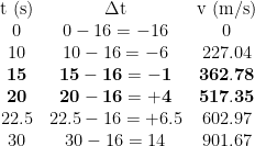
We can first look at a single data point and interpolate using its value. If the nearest datapoint does not differ much from the value being estimated it can be a good enough estimate in some cases. In this case the nearest datapoint is t=15, so we just take the value from it.

$\displaystyle \begin{array}{*{20}{c}} {\text{t (s)}} & {\Delta \text{t}} & {\text{v (m/s)}} \\ 0 & {0-16=-16} & 0 \\ {10} & {10-16=-6} & {227.04} \\ \mathbf{15} & \mathbf{15-16=-1} & \mathbf{362.78} \\ {20} & {20-16=+4} & {517.35} \\ {22.5} & {22.5-16=+6.5} & {602.97} \\ {30} & {30-16=14} & {901.67} \end{array}$

This is the 2nd index of the vector t and v, so we just use our single time point t[2] and its velocity v[2] to guess the value when t=16.

# Perquisites
import numpy as np
import scipy as sp
import matplotlib.pyplot as plt
import scipy.interpolate
# Create Data
t=np.array([0,10,15,20,22.5,30])
v=np.array([0,227.04,362.78,517.35,602.97,901.67])
# Plot Data
plt.close('all')
plt.figure(1)
plt.grid(axis='both',which='major',color=[166/255,166/255,166/255], linestyle='-', linewidth=2)
plt.minorticks_on()
plt.grid(axis='both',which='minor',color=[166/255,166/255,166/255], linestyle=':', linewidth=1)
plt.xlabel('time (s)')         
plt.ylabel('velocity (m/s)')        
plt.title('Projectile of a Rocket') 
plt.scatter(t,v,50,[255/255,0/255,0/255],label='original data')
plt.legend(loc='upper left')
# Data Point to be Interpolated
plt.plot([16, 16], [0, np.max(v)], color=[0/255,176/255,80/255], linestyle=':', linewidth=2)
# Nearest Point Interpolation
tnear=15
vnear=v[2]
t16_near=16
v16_near=vnear
print(v16_near)

362.78

Using this data, the plot can be made using the code:

# Perquisites
import numpy as np
import scipy as sp
import matplotlib.pyplot as plt
import scipy.interpolate
# Create Data
t=np.array([0,10,15,20,22.5,30])
v=np.array([0,227.04,362.78,517.35,602.97,901.67])
# Plot Data
plt.close('all')
plt.figure(1)
plt.grid(axis='both',which='major',color=[166/255,166/255,166/255], linestyle='-', linewidth=2)
plt.minorticks_on()
plt.grid(axis='both',which='minor',color=[166/255,166/255,166/255], linestyle=':', linewidth=1)
plt.xlabel('time (s)')         
plt.ylabel('velocity (m/s)')        
plt.title('Projectile of a Rocket') 
plt.scatter(t,v,50,[255/255,0/255,0/255],label='original data')
# Data Point to be Interpolated
plt.plot([16, 16], [0, np.max(v)], color=[0/255,176/255,80/255], linestyle=':', linewidth=2)
# Nearest Point Interpolation
tnear=15
vnear=v[2]
t16_near=16
v16_near=vnear
# Add Nearest Datapoint to Plot
plt.scatter(16,v16_near,50,color=[0/255,112/255,192/255],
            label='nearest point interpolation')
plt.legend(loc='upper left')

Linear Interpolation

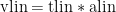
For Linear Interpolation we need to use 2 datapoints, these should be the nearest 2 datapoints to time point we are interested in namely in this case t=15 and t=20, the 2nd and 3rd index of t and v

$\displaystyle \begin{array}{*{20}{c}} {\text{t (s)}} & {\Delta \text{t}} & {\text{v (m/s)}} \\ 0 & {0-16=-16} & 0 \\ {10} & {10-16=-6} & {227.04} \\ \mathbf{15} & \mathbf{15-16=-1} & \mathbf{362.78} \\ \mathbf{20} & \mathbf{20-16=+4} & \mathbf{517.35} \\ {22.5} & {22.5-16=+6.5} & {602.97} \\ {30} & {30-16=14} & {901.67} \end{array}$

Here instead of referencing only the nearest data point, we reference the nearest 2 data points, we then fit a line between them and calculate the value of v on the line at t=16 and use that as our estimate for v[16].

The equation for a straight line is:

$\displaystyle v[t]={{a}_{0}}+{{a}_{1}}*t$

To solve for 2 unknowns:

$\displaystyle {{a}_{0}},{{a}_{1}}$

We require 2 equations:

$\displaystyle \left[ {\begin{array}{*{20}{c}} {{{v}_{0}}} \\ {{{v}_{1}}} \end{array}} \right]=\left[ {\begin{array}{*{20}{c}} 1 & {15} \\ 1 & {20} \end{array}} \right]*\left[ {\begin{array}{*{20}{c}} {{{a}_{0}}} \\ {{{a}_{1}}} \end{array}} \right]$

Inputting our known values:

$\displaystyle \left[ {\begin{array}{*{20}{c}} {362.78} \\ {517.35} \end{array}} \right]=\left[ {\begin{array}{*{20}{c}} 1 & {15} \\ 1 & {20} \end{array}} \right]*\left[ {\begin{array}{*{20}{c}} {{{a}_{0}}} \\ {{{a}_{1}}} \end{array}} \right]$

Creating these 3 as matrices:

$\displaystyle \text{vlin}=\left[ {\begin{array}{*{20}{c}} {362.78} \\ {517.35} \end{array}} \right]$

$\displaystyle \text{tlin}=\left[ {\begin{array}{*{20}{c}} 1 & {15} \\ 1 & {20} \end{array}} \right]$

$\displaystyle \text{alin}=\left[ {\begin{array}{*{20}{c}} {{{a}_{0}}} \\ {{{a}_{1}}} \end{array}} \right]$

We can re-write the above:

$\displaystyle \text{vlin}=\text{tlin}*\text{alin}$

Solving for alin:

$\displaystyle \text{inv(tlin)}*\text{vlin}=\text{inv(tlin)}*\text{tlin}*\text{alin}$

Where:

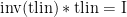
$\displaystyle \text{inv(tlin)}*\text{tlin}=\text{I}$

$\displaystyle \text{inv(tlin)}*\text{vlin}=\text{alin}$

Rearranging:

$\displaystyle \text{alin}=\text{inv(tlin)}*\text{vlin}$

Once we have these coefficients, it is simply a case of inserting them into the equation at t=16:

$\displaystyle \text{v16lin}=\left[ {\begin{array}{*{20}{c}} 1 & {16} \end{array}} \right]*\text{alin}$

We can do these steps in Python by using the 2nd and 3rd index of t to create our tlin matrix and the 2nd and 3rd index of v to create our vlin vector.

# Perquisites
import numpy as np
import scipy as sp
import matplotlib.pyplot as plt
import scipy.interpolate
# Create Data
t=np.array([0,10,15,20,22.5,30])
v=np.array([0,227.04,362.78,517.35,602.97,901.67])
# Plot Data
plt.close('all')
plt.figure(1)
plt.grid(axis='both',which='major',color=[166/255,166/255,166/255], linestyle='-', linewidth=2)
plt.minorticks_on()
plt.grid(axis='both',which='minor',color=[166/255,166/255,166/255], linestyle=':', linewidth=1)
plt.xlabel('time (s)')         
plt.ylabel('velocity (m/s)')        
plt.title('Projectile of a Rocket') 
plt.scatter(t,v,50,[255/255,0/255,0/255],label='original data')
# Data Point to be Interpolated
plt.plot([16, 16], [0, np.max(v)], color=[0/255,176/255,80/255], linestyle=':', linewidth=2)
# Nearest Point Interpolation
tnear=15
vnear=v[2]
t16_near=16
v16_near=vnear
# Linear Interpolation
tlin=np.array([[1,t[2]],
               [1,t[3]]])
vlin=v[[2,3]]
print(tlin)
print(vlin)

[[ 1. 15.]
 [ 1. 20.]]

[362.78 517.35]

We can solve to get the coefficients, alin by using the linear algebra library. We can first of all calculate the inverse of the square matrix tlin and then use this to perform array multiplication on the vector vlin, alternatively we can use the function solve from the linear algebra library, which employs the same method, calculating the inverse of tlin in the background and finally we can also use the least square method to calculate the coefficients of alin.

# Perquisites
import numpy as np
import scipy as sp
import matplotlib.pyplot as plt
import scipy.interpolate
# Create Data
t=np.array([0,10,15,20,22.5,30])
v=np.array([0,227.04,362.78,517.35,602.97,901.67])
# Plot Data
plt.close('all')
plt.figure(1)
plt.grid(axis='both',which='major',color=[166/255,166/255,166/255], linestyle='-', linewidth=2)
plt.minorticks_on()
plt.grid(axis='both',which='minor',color=[166/255,166/255,166/255], linestyle=':', linewidth=1)
plt.xlabel('time (s)')         
plt.ylabel('velocity (m/s)')        
plt.title('Projectile of a Rocket') 
plt.scatter(t,v,50,[255/255,0/255,0/255],label='original data')
# Data Point to be Interpolated
plt.plot([16, 16], [0, np.max(v)], color=[0/255,176/255,80/255], linestyle=':', linewidth=2)
# Nearest Point Interpolation
t16_nearest=16
v16_nearest=v[2]
# Linear Interpolation
tnear=15
vnear=v[2]
t16_near=16
v16_near=vnear
# Solve using Inverse Matrix
tlin_inv=np.linalg.inv(tlin)
alin_a=np.linalg.inv(tlin)@vlin
# Solve using Solve (Uses Inverse Matrix - Only Works with Square Matrices)
alin_b=np.linalg.solve(tlin,vlin)
# Solve Using Linear Least Squares
[alin_c,resid,rank,s] =np.linalg.lstsq(tlin,vlin,rcond=0)
# Print
print(alin_a)
print(alin_b)
print(alin_c)

For a simple set of equations, all three methods yield the same result.

[-100.93    30.914]
[-100.93    30.914]
[-100.93    30.914]

Once alin is calculated we can use it to perform array multiplication on a t16_lin vector.

# Perquisites
import numpy as np
import scipy as sp
import matplotlib.pyplot as plt
import scipy.interpolate
# Create Data
t=np.array([0,10,15,20,22.5,30])
v=np.array([0,227.04,362.78,517.35,602.97,901.67])
# Plot Data
plt.close('all')
plt.figure(1)
plt.grid(axis='both',which='major',color=[166/255,166/255,166/255], linestyle='-', linewidth=2)
plt.minorticks_on()
plt.grid(axis='both',which='minor',color=[166/255,166/255,166/255], linestyle=':', linewidth=1)
plt.xlabel('time (s)')         
plt.ylabel('velocity (m/s)')        
plt.title('Projectile of a Rocket') 
plt.scatter(t,v,50,[255/255,0/255,0/255],label='original data')
# Data Point to be Interpolated
plt.plot([16, 16], [0, np.max(v)], color=[0/255,176/255,80/255], linestyle=':', linewidth=2)
# Nearest Point Interpolation
tnear=15
vnear=v[2]
t16_near=16
v16_near=vnear
# Linear Interpolation
tlin=np.array([[1,t[2]],
               [1,t[3]]])
vlin=v[[2,3]]
alin=np.linalg.solve(tlin,vlin)
t16_lin=[1,16]
v16_lin=alin@t16_lin
v16_lin=np.round(v16_lin,3)
print(v16_lin)

393.694

The linear line with coefficients a0 and a1 will in only work well in most cases, within the specified lower and upper bound, in this case in the regime between t=15 and t=20. Attempting to use the equation to interpolate values at t=0 and t=30 gives:

# Perquisites
import numpy as np
import scipy as sp
import matplotlib.pyplot as plt
import scipy.interpolate
# Create Data
t=np.array([0,10,15,20,22.5,30])
v=np.array([0,227.04,362.78,517.35,602.97,901.67])
# Plot Data
plt.close('all')
plt.figure(1)
plt.grid(axis='both',which='major',color=[166/255,166/255,166/255], linestyle='-', linewidth=2)
plt.minorticks_on()
plt.grid(axis='both',which='minor',color=[166/255,166/255,166/255], linestyle=':', linewidth=1)
plt.xlabel('time (s)')         
plt.ylabel('velocity (m/s)')        
plt.title('Projectile of a Rocket') 
plt.scatter(t,v,50,[255/255,0/255,0/255],label='original data')
# Data Point to be Interpolated
plt.plot([16, 16], [0, np.max(v)], color=[0/255,176/255,80/255], linestyle=':', linewidth=2)
# Nearest Point Interpolation
tnear=15
vnear=v[2]
t16_near=16
v16_near=vnear
# Linear Interpolation
tlin=np.array([[1,t[2]],
               [1,t[3]]])
vlin=v[[2,3]]
alin=np.linalg.solve(tlin,vlin)
t16_lin=[1,16]
v16_lin=alin@t16_lin
v16_lin=np.round(v16_lin,3)
# Linear Interpolation Plot
plt.scatter(16,v16_lin,50,color=[255/255,192/255,0/255],label='linear interpolation')
plt.legend(loc='upper left')
# Use alin on End Datapoints
t0_lin=[1,0]
v0_lin=alin@t0_lin
t30_lin=[1,30]
v30_lin=alin@t30_lin
print(t0_lin)
print(v0_lin)
print(t30_lin)
print(v30_lin)

[1, 0]
-100.93000000000028

[1, 30]
826.4900000000001

The v0_lin value is well out the 0,0 value of the origin which we were given, while the v30_lin is also lower than the last value we were given in our data set. These can be plotted with respect to one another:

# Perquisites
import numpy as np
import scipy as sp
import matplotlib.pyplot as plt
import scipy.interpolate
# Create Data
t=np.array([0,10,15,20,22.5,30])
v=np.array([0,227.04,362.78,517.35,602.97,901.67])
# Plot Data
plt.close('all')
plt.figure(1)
plt.grid(axis='both',which='major',color=[166/255,166/255,166/255], linestyle='-', linewidth=2)
plt.minorticks_on()
plt.grid(axis='both',which='minor',color=[166/255,166/255,166/255], linestyle=':', linewidth=1)
plt.xlabel('time (s)')         
plt.ylabel('velocity (m/s)')        
plt.title('Projectile of a Rocket') 
plt.scatter(t,v,50,[255/255,0/255,0/255],label='original data')
# Data Point to be Interpolated
plt.plot([16, 16], [0, np.max(v)], color=[0/255,176/255,80/255], linestyle=':', linewidth=2)
# Nearest Point Interpolation
tnear=15
vnear=v[2]
t16_near=16
v16_near=vnear
# Linear Interpolation
tlin=np.array([[1,t[2]],
               [1,t[3]]])
vlin=v[[2,3]]
alin=np.linalg.solve(tlin,vlin)
t16_lin=[1,16]
v16_lin=alin@t16_lin
v16_lin=np.round(v16_lin,3)
# Linear Interpolation Plot
plt.scatter(16,v16_lin,50,color=[255/255,192/255,0/255],label='linear interpolation')
plt.legend(loc='upper left')
# Use alin on End Datapoints
t0_lin=[1,0]
v0_lin=alin@t0_lin
t30_lin=[1,30]
v30_lin=alin@t30_lin
# Add Straight Line
plt.plot([t[0], t[5]], [v0_lin, v30_lin], color=[0/255,112/255,192/255], linestyle=':', linewidth=2)
# Add Acatter of v16_lin 
plt.scatter(16,v16_lin,50,color=[255/255,192/255,0/255],label='linear interpolation')

Quadratic Interpolation

For quadratic interpolation, we interpolate using the nearest 3 data points, in the case of t=16, this is t=15, t=20 and t=10. we then fit a quadratic curve between them and calculate the value of v on the line at t=16 and use that as our estimate for v[16]:

$\displaystyle \begin{array}{*{20}{c}} {\text{t (s)}} & {\Delta \text{t}} & {\text{v (m/s)}} \\ 0 & {0-16=-16} & 0 \\ \mathbf{10} & \mathbf{10-16=-6} & \mathbf{227.04} \\ \mathbf{15} & \mathbf{15-16=-1} & \mathbf{362.78} \\ \mathbf{20} & \mathbf{20-16=+4} & \mathbf{517.35} \\ {22.5} & {22.5-16=+6.5} & {602.97} \\ {30} & {30-16=14} & {901.67} \end{array}$

The equation for a quadratic curve is:

$\displaystyle v[t]={{a}_{0}}+{{a}_{1}}*t+{{a}_{2}}*{{t}^{2}}$

To solve for 3 unknowns:

$\displaystyle {{a}_{0}},{{a}_{1}},{{a}_{2}}$

We require 3 equations:

$\displaystyle \left[ {\begin{array}{*{20}{c}} {{{v}_{0}}} \\ {{{v}_{1}}} \\ {{{v}_{2}}} \end{array}} \right]=\left[ {\begin{array}{*{20}{c}} 1 & {{{v}_{0}}} & {v_{0}^{2}} \\ 1 & {{{v}_{1}}} & {v_{1}^{2}} \\ 1 & {{{v}_{2}}} & {v_{2}^{2}} \end{array}} \right]*\left[ {\begin{array}{*{20}{c}} {{{a}_{0}}} \\ {{{a}_{1}}} \\ {{{a}_{2}}} \end{array}} \right]$

Inputting our known values:

$\displaystyle \left[ {\begin{array}{*{20}{c}} {10} \\ {15} \\ {20} \end{array}} \right]=\left[ {\begin{array}{*{20}{c}} 1 & {10} & {{{{10}}^{2}}} \\ 1 & {15} & {{{{15}}^{2}}} \\ 1 & {20} & {{{{20}}^{2}}} \end{array}} \right]*\left[ {\begin{array}{*{20}{c}} {{{a}_{0}}} \\ {{{a}_{1}}} \\ {{{a}_{2}}} \end{array}} \right]$

Creating these 3 as matrices:

$\displaystyle \text{vquad}=\left[ {\begin{array}{*{20}{c}} {10} \\ {15} \\ {20} \end{array}} \right]$

$\displaystyle \text{tquad}=\left[ {\begin{array}{*{20}{c}} 1 & {10} & {{{{10}}^{2}}} \\ 1 & {15} & {{{{15}}^{2}}} \\ 1 & {20} & {{{{20}}^{2}}} \end{array}} \right]$

$\displaystyle \text{aquad=}\left[ {\begin{array}{*{20}{c}} {{{a}_{0}}} \\ {{{a}_{1}}} \\ {{{a}_{2}}} \end{array}} \right]$

We can re-write the above:

$\displaystyle \text{vquad}=\text{tquad}*\text{aquad}$

Solving for aquad using the inverse:

$\displaystyle \text{aquad}=\text{inv}\left( {\text{tquad}} \right)*\text{vquad}$

Once we have these coefficients it is simply a case of inserting them into the equation at t=16:

$\displaystyle \text{v16quad}=\left[ {\begin{array}{*{20}{c}} 1 & {16} & {{{{16}}^{2}}} \end{array}} \right]*\text{aquad}$

We can do these steps in Python by using the 1st, 2nd and 3rd index of t to create our tquad matrix and the 1st, 2nd and 3rd index of v to create our vquad vector. We can solve to get the coefficients, aquad by using solve from the linear algebra library and perform array multiplication with the t16_quad vector to get our interpolated value.

# Perquisites
import numpy as np
import scipy as sp
import matplotlib.pyplot as plt
import scipy.interpolate
# Create Data
t=np.array([0,10,15,20,22.5,30])
v=np.array([0,227.04,362.78,517.35,602.97,901.67])
# Plot Data
plt.close('all')
plt.figure(1)
plt.grid(axis='both',which='major',color=[166/255,166/255,166/255], linestyle='-', linewidth=2)
plt.minorticks_on()
plt.grid(axis='both',which='minor',color=[166/255,166/255,166/255], linestyle=':', linewidth=1)
plt.xlabel('time (s)')         
plt.ylabel('velocity (m/s)')        
plt.title('Projectile of a Rocket') 
plt.scatter(t,v,50,[255/255,0/255,0/255],label='original data')
# Data Point to be Interpolated
plt.plot([16, 16], [0, np.max(v)], color=[0/255,176/255,80/255], linestyle=':', linewidth=2)
# Nearest Point Interpolation
tnear=15
vnear=v[2]
t16_near=16
v16_near=vnear
# Linear Interpolation
tlin=np.array([[1,t[2]],
               [1,t[3]]])
vlin=v[[2,3]]
alin=np.linalg.solve(tlin,vlin)
t16_lin=[1,16]
v16_lin=alin@t16_lin
v16_lin=np.round(v16_lin,3)
# Quadratic Interpolation
tquad=np.array([[1,t[1],t[1]**2],
                [1,t[2],t[2]**2],
                [1,t[3],t[3]**2]])
vquad=v[[1,2,3]]
aquad=np.linalg.solve(tquad,vquad)
t16_quad=[1,16,16**2]
v16_quad=aquad@t16_quad
v16_quad=np.round(v16_quad,3)

392.188

Cubic Interpolation

For cubic interpolation, we interpolate using the nearest 4 data points, in the case of t=16, this is t=15, t=20 and t=10. we then fit a quadratic curve between them and calculate the value of v on the line at t=16 and use that as our estimate for v[16]:

$\displaystyle \begin{array}{*{20}{c}} {\text{t (s)}} & {\Delta \text{t}} & {\text{v (m/s)}} \\ 0 & {0-16=-16} & 0 \\ \mathbf{10} & \mathbf{10-16=-6} & \mathbf{227.04} \\ \mathbf{15} & \mathbf{15-16=-1} & \mathbf{362.78} \\ \mathbf{20} & \mathbf{20-16=+4} & \mathbf{517.35} \\ \mathbf{22.5} & \mathbf{22.5-16=+6.5} & \mathbf{602.97} \\ {30} & {30-16=14} & {901.67} \end{array}$

The equation for a cubic function is:

$\displaystyle v[t]={{a}_{0}}+{{a}_{1}}*t+{{a}_{2}}*{{t}^{2}}+{{a}_{3}}*{{t}^{3}}$

To solve for 4 unknowns:

$\displaystyle {{a}_{0}},{{a}_{1}},{{a}_{2}},{{a}_{3}}$

We require 4 equations:

$\displaystyle \left[ {\begin{array}{*{20}{c}} {{{v}_{0}}} \\ {{{v}_{1}}} \\ {{{v}_{2}}} \\ {{{v}_{3}}} \end{array}} \right]=\left[ {\begin{array}{*{20}{c}} 1 & {{{t}_{0}}} & {t_{0}^{2}} & {t_{0}^{3}} \\ 1 & {{{t}_{1}}} & {t_{1}^{2}} & {t_{1}^{3}} \\ 1 & {{{t}_{2}}} & {t_{2}^{2}} & {t_{2}^{3}} \\ 1 & {{{t}_{3}}} & {t_{3}^{2}} & {t_{3}^{3}} \end{array}} \right]*\left[ {\begin{array}{*{20}{c}} {{{a}_{0}}} \\ {{{a}_{1}}} \\ {{{a}_{2}}} \\ {{{a}_{3}}} \end{array}} \right]$

Inputting our known values:

$\displaystyle \left[ {\begin{array}{*{20}{c}} {227.04} \\ {362.78} \\ {517.35} \\ {602.97} \end{array}} \right]=\left[ {\begin{array}{*{20}{c}} 1 & {10} & {{{{10}}^{2}}} & {{{{10}}^{2}}} \\ 1 & {15} & {{{{15}}^{2}}} & {{{{15}}^{3}}} \\ 1 & {20} & {{{{20}}^{2}}} & {{{{20}}^{3}}} \\ 1 & {22.5} & {{{{22.5}}^{2}}} & {{{{22.5}}^{3}}} \end{array}} \right]*\left[ {\begin{array}{*{20}{c}} {{{a}_{0}}} \\ {{{a}_{1}}} \\ {{{a}_{2}}} \\ {{{a}_{3}}} \end{array}} \right]$

Creating these 3 as matrices:

$\displaystyle \text{vcubic}=\left[ {\begin{array}{*{20}{c}} {10} \\ {15} \\ {20} \\ {22.5} \end{array}} \right]$

$\displaystyle \text{tcubic=}\left[ {\begin{array}{*{20}{c}} 1 & {10} & {{{{10}}^{2}}} & {{{{10}}^{3}}} \\ 1 & {15} & {{{{15}}^{2}}} & {{{{15}}^{3}}} \\ 1 & {20} & {{{{20}}^{2}}} & {{{{20}}^{3}}} \\ 1 & {22.5} & {{{{22.5}}^{2}}} & {{{{22.5}}^{3}}} \end{array}} \right]$

$\displaystyle \text{acubic=}\left[ {\begin{array}{*{20}{c}} {{{a}_{0}}} \\ {{{a}_{1}}} \\ {{{a}_{2}}} \\ {{{a}_{3}}} \end{array}} \right]$

We can re-write the above:

$\displaystyle \text{vcubic}=\text{tcubic}*\text{acubic}$

Solving for a cubic function using the inverse:

$\displaystyle \text{acubic}=\text{inv}\left( {\text{tcubic}} \right)*\text{vcubic}$

Once we have these, it is simply a case of inserting them into the equation at t=16:

$\displaystyle \text{v16cubic}=\left[ {\begin{array}{*{20}{c}} 1 & {16} & {{{{16}}^{2}}} & {{{{16}}^{3}}} \end{array}} \right]*\text{acubic}$

We can do these steps in Python by using the 1st, 2nd, 3rd and 4th index of t to create our tcubic matrix and the 1st, 2nd, 3rd and 4th index of v to create our vcubicvector. We can solve to get the coefficients, acubic by using solve from the linear algebra library and perform array multiplication with the t16_cubic vector to get our interpolated value.

# Perquisites
import numpy as np
import scipy as sp
import matplotlib.pyplot as plt
import scipy.interpolate
# Create Data
t=np.array([0,10,15,20,22.5,30])
v=np.array([0,227.04,362.78,517.35,602.97,901.67])
# Plot Data
plt.close('all')
plt.figure(1)
plt.grid(axis='both',which='major',color=[166/255,166/255,166/255], linestyle='-', linewidth=2)
plt.minorticks_on()
plt.grid(axis='both',which='minor',color=[166/255,166/255,166/255], linestyle=':', linewidth=1)
plt.xlabel('time (s)')         
plt.ylabel('velocity (m/s)')        
plt.title('Projectile of a Rocket') 
plt.scatter(t,v,50,[255/255,0/255,0/255],label='original data')
# Data Point to be Interpolated
plt.plot([16, 16], [0, np.max(v)], color=[0/255,176/255,80/255], linestyle=':', linewidth=2)
# Nearest Point Interpolation
tnear=15
vnear=v[2]
t16_near=16
v16_near=vnear
# Linear Interpolation
tlin=np.array([[1,t[2]],
               [1,t[3]]])
vlin=v[[2,3]]
alin=np.linalg.solve(tlin,vlin)
t16_lin=[1,16]
v16_lin=alin@t16_lin
v16_lin=np.round(v16_lin,3)
# Quadratic Interpolation
tquad=np.array([[1,t[1],t[1]**2],
                [1,t[2],t[2]**2],
                [1,t[3],t[3]**2]])
vquad=v[[1,2,3]]
aquad=np.linalg.solve(tquad,vquad)
t16_quad=[1,16,16**2]
v16_quad=aquad@t16_quad
v16_quad=np.round(v16_quad,3)
# Cubic Interpolation
tcubic=np.array([[1,t[1],t[1]**2,t[1]**3],
                [1,t[2],t[2]**2,t[2]**3],
                [1,t[3],t[3]**2,t[3]**3],
                [1,t[4],t[4]**2,t[4]**3]])
vcubic=v[[1,2,3,4]]
acubic=np.linalg.solve(tcubic,vcubic)
t16_cubic=[1,16,16**2,16**3]
v16_cubic=acubic@t16_cubic
v16_cubic=np.round(v16_cubic,3)
print(v16_cubic)

392.057

Comparison

As we can see with the more data points used the value begins to converge:

$\displaystyle \begin{array}{*{20}{c}} {\text{Method}} & {\text{t}\left[ {16} \right]} \\ {\text{nearest}} & {362.78} \\ {\text{linear}} & {393.694} \\ {\text{quadratic}} & {392.188} \\ {\text{cubic}} & {392.057} \end{array}$

Interpolation of Multiple Data Points using an Interpolation Function

To use the interpolation function we need to import the scipy.interpolate library (line 5).

Nearest Point Interpolation

To interpolate, we must first create an interpolation function from the existing x and y (in this case t and v) data. We can do this by loading interp1d from the interpolate library of SciPy. For the input arguments, we specify our origina x and y co-ordinates and we specify the method as a keyword input argument, in this case we will select the method nearest:

# Perquisites
import numpy as np
import scipy as sp
import matplotlib.pyplot as plt
import scipy.interpolate
# Create Data
t=np.array([0,10,15,20,22.5,30])
v=np.array([0,227.04,362.78,517.35,602.97,901.67])
# Plot Data
plt.close('all')
plt.figure(1)
plt.grid(axis='both',which='major',color=[166/255,166/255,166/255], linestyle='-', linewidth=2)
plt.minorticks_on()
plt.grid(axis='both',which='minor',color=[166/255,166/255,166/255], linestyle=':', linewidth=1)
plt.xlabel('time (s)')         
plt.ylabel('velocity (m/s)')        
plt.title('Projectile of a Rocket') 
plt.scatter(t,v,50,[255/255,0/255,0/255],label='original data')
# Create an Interpolation Function
fvnearest=sp.interpolate.interp1d(t,v,kind='nearest')

Next we must specify new x values. In this case we want to create a variable tnew which starts from 0 and ends at 30 consisting of integer values, we can use the function arange to do this:

# Perquisites
import numpy as np
import scipy as sp
import matplotlib.pyplot as plt
import scipy.interpolate
# Create Data
t=np.array([0,10,15,20,22.5,30])
v=np.array([0,227.04,362.78,517.35,602.97,901.67])
# Plot Data
plt.close('all')
plt.figure(1)
plt.grid(axis='both',which='major',color=[166/255,166/255,166/255], linestyle='-', linewidth=2)
plt.minorticks_on()
plt.grid(axis='both',which='minor',color=[166/255,166/255,166/255], linestyle=':', linewidth=1)
plt.xlabel('time (s)')         
plt.ylabel('velocity (m/s)')        
plt.title('Projectile of a Rocket') 
plt.scatter(t,v,50,[255/255,0/255,0/255],label='original data')
# Create an Interpolation Function
fvnearest=sp.interpolate.interp1d(t,v,kind='nearest')
# Create New x Datapoints
tnew=np.arange(start=0,stop=30,step=1)
print(tnew)

[ 0  1  2  3  4  5  6  7  8  9 10 11 12 13 14 15 16 17 18 19 20 21 22 23 24 25 26 27 28 29]

To get the y values at these x values, we assign them as an input argument into our created interpolation function. In our case our new x values are tnew, we can calculate vnearest by using the nearest interpolation function fvnearest with tnew as an input argument:

# Perquisites
import numpy as np
import scipy as sp
import matplotlib.pyplot as plt
import scipy.interpolate
# Create Data
t=np.array([0,10,15,20,22.5,30])
v=np.array([0,227.04,362.78,517.35,602.97,901.67])
# Plot Data
plt.close('all')
plt.figure(1)
plt.grid(axis='both',which='major',color=[166/255,166/255,166/255], linestyle='-', linewidth=2)
plt.minorticks_on()
plt.grid(axis='both',which='minor',color=[166/255,166/255,166/255], linestyle=':', linewidth=1)
plt.xlabel('time (s)')         
plt.ylabel('velocity (m/s)')        
plt.title('Projectile of a Rocket') 
plt.scatter(t,v,50,[255/255,0/255,0/255],label='original data')
# Create an Interpolation Function
fvnearest=sp.interpolate.interp1d(t,v,kind='nearest')
# Create tnew Datapoints
tnew=np.arange(start=0,stop=30,step=1)
# Generate Interpolated vnearest Data at tnew
vnearest=fvnearest(tnew)
print(vnearest)

[  0.     0.     0.     0.     0.     0.   227.04 227.04 227.04 227.04 227.04 227.04 227.04 362.78 362.78 362.78 362.78 362.78 517.35 517.35 517.35 517.35 602.97 602.97 602.97 602.97 602.97 901.67 901.67 901.67]

Of course before we calculated manually the value at v16nearest earlier we can compare this to the value of vnearest[16]

# Perquisites
import numpy as np
import scipy as sp
import matplotlib.pyplot as plt
import scipy.interpolate
# Create Data
t=np.array([0,10,15,20,22.5,30])
v=np.array([0,227.04,362.78,517.35,602.97,901.67])
# Plot Data
plt.close('all')
plt.figure(1)
plt.grid(axis='both',which='major',color=[166/255,166/255,166/255], linestyle='-', linewidth=2)
plt.minorticks_on()
plt.grid(axis='both',which='minor',color=[166/255,166/255,166/255], linestyle=':', linewidth=1)
plt.xlabel('time (s)')         
plt.ylabel('velocity (m/s)')        
plt.title('Projectile of a Rocket') 
plt.scatter(t,v,50,[255/255,0/255,0/255],label='original data')
# Create an Interpolation Function
fvnearest=sp.interpolate.interp1d(t,v,kind='nearest')
# Create tnew Datapoints
tnew=np.arange(start=0,stop=30,step=1)
# Generate Interpolated vnearest Data at tnew
vnearest=fvnearest(tnew)
print(vnearest[16])

362.78

We can plot out these values with respect to the original data

# Perquisites
import numpy as np
import scipy as sp
import matplotlib.pyplot as plt
import scipy.interpolate
# Create Data
t=np.array([0,10,15,20,22.5,30])
v=np.array([0,227.04,362.78,517.35,602.97,901.67])
# Plot Data
plt.close('all')
plt.figure(1)
plt.grid(axis='both',which='major',color=[166/255,166/255,166/255], linestyle='-', linewidth=2)
plt.minorticks_on()
plt.grid(axis='both',which='minor',color=[166/255,166/255,166/255], linestyle=':', linewidth=1)
plt.xlabel('time (s)')         
plt.ylabel('velocity (m/s)')        
plt.title('Projectile of a Rocket') 
plt.scatter(t,v,50,[255/255,0/255,0/255],label='original data')
# Create an Interpolation Function
fvnearest=sp.interpolate.interp1d(t,v,kind='nearest')
# Create tnew Datapoints
tnew=np.arange(start=0,stop=30,step=1)
# Generate Interpolated vnearest Data at tnew
vnearest=fvnearest(tnew)
# Add tnew, vnearest line to existing plot
plt.plot(tnew,vnearest,color=[0/255,112/255,192/255], linestyle=':',label='nearest interpolation')
plt.legend(loc='upper left')

Linear Interpolation

The form for Linear interpolation is the same for the Nearest interpolation except for the fact that we use linear as the kind. We can print the value out at t=16:

# Perquisites
import numpy as np
import scipy as sp
import matplotlib.pyplot as plt
import scipy.interpolate
# Create Data
t=np.array([0,10,15,20,22.5,30])
v=np.array([0,227.04,362.78,517.35,602.97,901.67])
# Plot Data
plt.close('all')
plt.figure(1)
plt.grid(axis='both',which='major',color=[166/255,166/255,166/255], linestyle='-', linewidth=2)
plt.minorticks_on()
plt.grid(axis='both',which='minor',color=[166/255,166/255,166/255], linestyle=':', linewidth=1)
plt.xlabel('time (s)')         
plt.ylabel('velocity (m/s)')        
plt.title('Projectile of a Rocket') 
plt.scatter(t,v,50,[255/255,0/255,0/255],label='original data')
# Create tnew Datapoints
tnew=np.arange(start=0,stop=30,step=1)
# Nearest Interpolation
fvnearest=sp.interpolate.interp1d(t,v,kind='nearest')
vnearest=fvnearest(tnew)
# Linear Interpolation
fvlinear=sp.interpolate.interp1d(t,v,kind='linear')
vlinear=fvlinear(tnew)
print(np.round(vlinear[16],3))
# Add tnew, vlinear line to existing plot
plt.plot(tnew,vlinear,color=[0/255,112/255,192/255], linestyle=':',label='linear interpolation')
plt.legend(loc='upper left')

393.694

And once again we see it matches what we manually calculated.

Quadratic Interpolation

Once again the procedure for quadratic interpolation is the same for the Nearest interpolation except for the fact that we use linear as the kind. We can print the value out at t=16:

# Perquisites
import numpy as np
import scipy as sp
import matplotlib.pyplot as plt
import scipy.interpolate
# Create Data
t=np.array([0,10,15,20,22.5,30])
v=np.array([0,227.04,362.78,517.35,602.97,901.67])
# Plot Data
plt.close('all')
plt.figure(1)
plt.grid(axis='both',which='major',color=[166/255,166/255,166/255], linestyle='-', linewidth=2)
plt.minorticks_on()
plt.grid(axis='both',which='minor',color=[166/255,166/255,166/255], linestyle=':', linewidth=1)
plt.xlabel('time (s)')         
plt.ylabel('velocity (m/s)')        
plt.title('Projectile of a Rocket') 
plt.scatter(t,v,50,[255/255,0/255,0/255],label='original data')
# Create tnew Datapoints
tnew=np.arange(start=0,stop=30,step=1)
# Nearest Interpolation
fvnearest=sp.interpolate.interp1d(t,v,kind='nearest')
vnearest=fvnearest(tnew)
# Linear Interpolation
fvlinear=sp.interpolate.interp1d(t,v,kind='linear')
vlinear=fvlinear(tnew)
# Quadratic Interpolation
fvquad=sp.interpolate.interp1d(t,v,kind='quadratic')
vquad=fvquad(tnew)
print(np.round(vquad[16],3))
# Add tnew, vquadratic line to existing plot
plt.plot(tnew,vquad,color=[0/255,112/255,192/255], linestyle=':',label='quadratic interpolation')
plt.legend(loc='upper left')

392.093

This is very similar to the value manually calculated (392.188) and any differences is likely to do with additional smoothing carried out when using the interpolation function.

Cubic Interpolation

Following out the form as used for the other methods of interpolation:

# Perquisites
import numpy as np
import scipy as sp
import matplotlib.pyplot as plt
import scipy.interpolate
# Create Data
t=np.array([0,10,15,20,22.5,30])
v=np.array([0,227.04,362.78,517.35,602.97,901.67])
# Plot Data
plt.close('all')
plt.figure(1)
plt.grid(axis='both',which='major',color=[166/255,166/255,166/255], linestyle='-', linewidth=2)
plt.minorticks_on()
plt.grid(axis='both',which='minor',color=[166/255,166/255,166/255], linestyle=':', linewidth=1)
plt.xlabel('time (s)')         
plt.ylabel('velocity (m/s)')        
plt.title('Projectile of a Rocket') 
plt.scatter(t,v,50,[255/255,0/255,0/255],label='original data')
# Create tnew Datapoints
tnew=np.arange(start=0,stop=30,step=1)
# Nearest Interpolation
fvnearest=sp.interpolate.interp1d(t,v,kind='nearest')
vnearest=fvnearest(tnew)
# Linear Interpolation
fvlinear=sp.interpolate.interp1d(t,v,kind='linear')
vlinear=fvlinear(tnew)
# Quadratic Interpolation
fvquad=sp.interpolate.interp1d(t,v,kind='quadratic')
vquad=fvquad(tnew)
# Cubic Interpolation
fvcubic=sp.interpolate.interp1d(t,v,kind='cubic')
vcubic=fvcubic(tnew)
print(np.round(vcubic[16],3))
# Add tnew, vcubic line to existing plot
plt.plot(tnew,vcubic,color=[0/255,112/255,192/255], linestyle=':',label='cubic interpolation')
plt.legend(loc='upper left')

392.071

This is once again very similar to the value manually calculated (392.071) and any differences is likely due to smoothing carried out by the interpolation function.

Tutorial Video

Perquisites

Data Points

Manual Interpolation of a Single Point

Nearest Point Interpolation

Linear Interpolation

Quadratic Interpolation

Cubic Interpolation

Comparison

Interpolation of Multiple Data Points using an Interpolation Function

Nearest Point Interpolation

Linear Interpolation

Quadratic Interpolation

Cubic Interpolation

Like this:

Leave a ReplyCancel reply

Tutorial Video

Perquisites

Data Points

Manual Interpolation of a Single Point

Nearest Point Interpolation

Linear Interpolation

Quadratic Interpolation

Cubic Interpolation

Comparison

Interpolation of Multiple Data Points using an Interpolation Function

Nearest Point Interpolation

Linear Interpolation

Quadratic Interpolation

Cubic Interpolation

Share this:

Like this:

Leave a ReplyCancel reply