Table of contents
Perquisites
Integration
Recall that we previously looked at numerical integration:
Starting off with a function for instance:


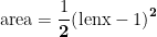
This yielded an area which was equal to:
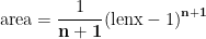
Or for a general power n
Let's have a look at the data in more detail by setting x and y as columns and concatenating them together as a matrix xy

Here the first column x, is the length across the x-axis and the second column y is the height of each bar. The total area is approximately the sum of all the bars. Lets look at the total area as we proceed along x and assign it as a new variable z. For the 0th row of z, we want the sum of the 0th element of y[0]. For the 1st row of z, we want the sum of the 0th element y[0] and 1st element y[1]. We can do this with a for loop, first we can create integers starting from 0 and using the length of y (line 1). We can then assign a new vector z to zeros using this length of y. In the for loop we can define i in integers and assign the ith index of z to the sum of y[0:i+1]. Note we need to use i+1 on the right hand side because we are using 0 order indexing. Recall with zero-order indexing we are going up to i but not reaching it so y[0:i] where i=0 means y[0:0] i.e. we are starting at i=0 and going to i=0 but not reaching it, which means we are summing no number and this would give us an additional 0 at the start. On the other hand y[0:i+1] where i=0 is y[0:1] and this is y[0].
This could also be done by creating z and initialising it to zeros, concatenating z to create xyz at the beginning and indexing within xyz using the for loop
Either case give the result:

z could also be calculated using the function cumsum.

Let's now go ahead and plot both y and z with respect to x as a scatter plot.

We see the function y=x increasing as x increases and the area under the curve z=int(y,x) increase as x increases. Here we have obtained the curve z from the existing x,y data. The inverse problem obtaining y from the plot of z, is known as differentiation. Let's have a look at this now.
Differentiation – Constant Term
Let's have a look at the plot of a constant term i.e.

Conceptually we can think of this as standing still and keeping the same position. Now let's create a straight line plot of this and let's also add a bar graph under the plot.

Instead of looking at the sum of each bar as we go along x we will look at the difference between the height of the bar with respect to the previous bar. Once again we can use a for loop to do this (line 10 and line 11).

Note when using this for loop, when i=0 line 11 becomes:
This looks at the last element of the array and subtracts it from the 0th element. This point is artificial and should be ignored. Because we are looking at the difference between points, we are actually one point less than we originally started. We can create new x values corresponding to this:
This gives

Note the function diff will also calculate this:
As expected z2a has the same dimensions as the first column in x2z2

The result is zeros across the board. This makes sense as the difference between a series of constants i.e. a constant minus itself is 0. Conceptually we can think of this as keeping a constant position and if we are keeping a constant position we aren't moving so have 0 speed. We can plot y with respect to x alongside z2 with respect to x2.

Differentiation – Linear Term
Let's have a look at the plot of a constant term i.e.
Conceptually we can think of this as moving a distance proportional to the time traveled, we know this should be a constant speed. Let's once again create a line plot of this and let's also add a bar graph under the plot.

Visually we can see that the plot is like a set of stairs and every step is a constant height. The difference between each step is therefore a constant. We can calculate this using the function diff.

As shown the step size is constant:

Once again we can plot x,y and x2,z2

Constant

Linear Power

Differentiation – Quadratic Term
Conceptually we can think of this as moving a distance proportional to the time traveled squared, we know this will increase our speed with respect to time (known as acceleration). Let's once again create a line plot of this and let's also add a bar graph under the plot.

Now if we calculate the difference between the bars:
This gives us:


And if we plot this out we can see:

Here we can see the straight line has the form of z=2x. We can now compare this to the earlier result
Constant

Linear Power

Quadratic Power

nth Power

Comparison: Integration and Differenciation
Let's compare figure 2 and figure 8, we can see they are really similar. Looking at the axes, we can see they differ by a scalar of 2.
Let us recreate the plot in Figure 2 but instead of using:

Let's look at:

Let's also overlay this on top of the plot of Figure 8.

As we can see the plots are almost identical, the difference between the plots is in the spacing and this is due to both sets of z data being inbetween points. For instance the x co-ordinate of the difference between y[1] and y[0] does not lie at x[0] but rather mid way between x[1] and x[0] which is x[0.5]. If line 6 and line 22 have the x values offset by 0.5.

And visually we can now see that integration and differentiation are inverse processes of one another.
We can think of integration as adding the sum of all the bars as we move from left to right – climbing the stairs.
And we can think of differentiation as being the difference in the bar height as we step down the stairs.
Uncertainty in Results
As we seen before with integration, the uncertainty in results is due to the finite bin width, due to there being some of the bars protruding above the curve and inversely some white space below the curve not occupied by a bar. The same applies to differentiation. Let's create a variable barwidth (line 1) which will be used to set the x co-ordinates (line 7). The z2 co-ordinates will be the difference in y values diff(y), normalised by the length of the difference in x which is the bar width (line 10). x2 can be created by using the length of the z2 co-ordinates and taking into account the step is now barwidth opposed to 1. The stop value is this the length of z2 multiplied by this bar width (line 11). The barwidth must also be specified in the function bar (line 16) to plot a bar graph with the desired width of bars.
With the barwidth (line 6) set to 1 the plots should remain unchanged from those seen earlier.


The barwidth can now be set to 0.5.


To 0.1


To 0.01


Exercise 1: Comparison Differentiation and Integration
Modify the code below and look at y=x**3 and z=diff(z,x) and compare this to y=3*x**2 and z=diff(y,x). These should once again be the inverse of one another. Repeat for y=x**4 and z=diff(z,x) and compare this to y=4*x**3 and z=diff(z,x).
Note if the code does not show, double click on the code block (it seems to be a bug with WordPress). All we need to do is change the equations in line 10 and line 30 as well as the labels in line 17 and line 37. We can optionally change the figure number (line 6).

Note if the code does not show, double click on the code block (it seems to be a bug with WordPress). All we need to do is change the equations in line 10 and line 30 as well as the labels in line 17 and line 37. We can optionally change the figure number (line 6).

Exercise 2: For Loop Practice
Exercises: Earlier we used the diff function (line 9) to calculate z2. Repeat this using a loop instead:
Note if the code does not show, double click on the code block (it seems to be a bug with WordPress).
